This project involved doing many different image processing techniques, most of which involved convolutions and/or filters in some way. It was a really interesting project, and I had a lot of fun applying the techniques taught in lecture to some of my own images. Every image used here, with the exception of the class examples and the blended picture with the Moon in the very last example, is a picture that I took myself.
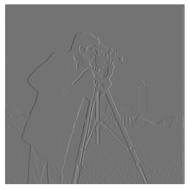
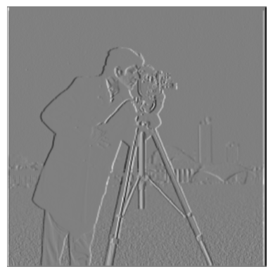
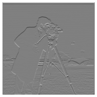
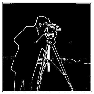
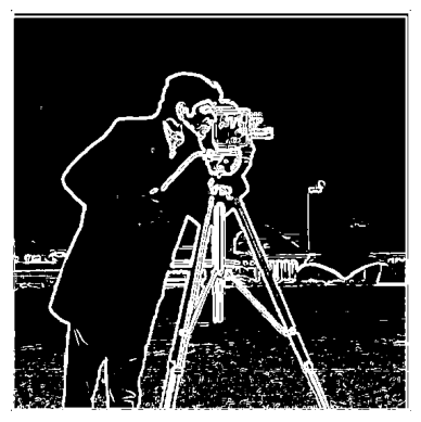
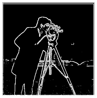
For this part, I used the finite difference operator to show the partial derivative in X and Y of the cameraman image. Specifically, I convolved the image with [1, -1] for dX, and with the transpose of [1, -1] for dY, to find the partial derivative images. Next, I found the gradient magnitude image by squaring both images and adding them together, and "binarized" this image by treating all pixels over a certain threshold as 1, and all others as 0.

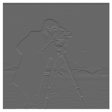
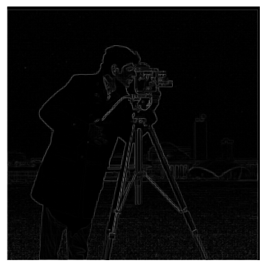
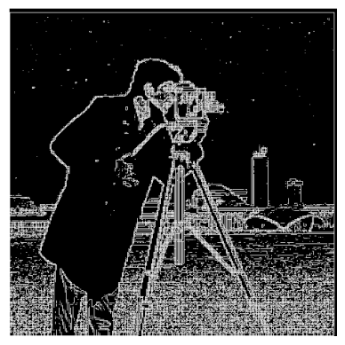
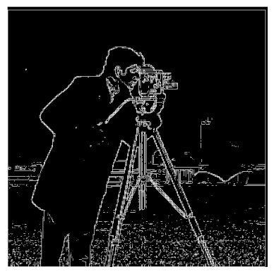
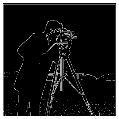
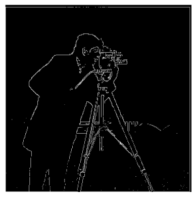
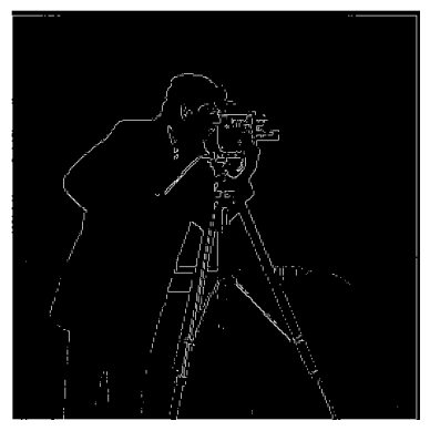

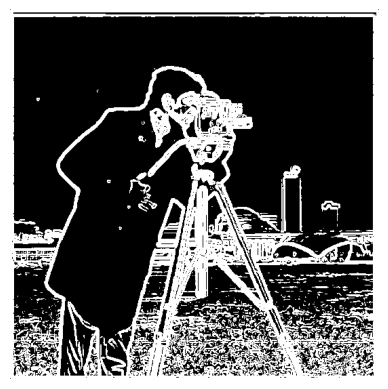
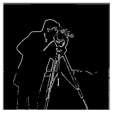
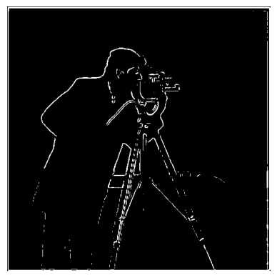
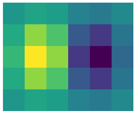
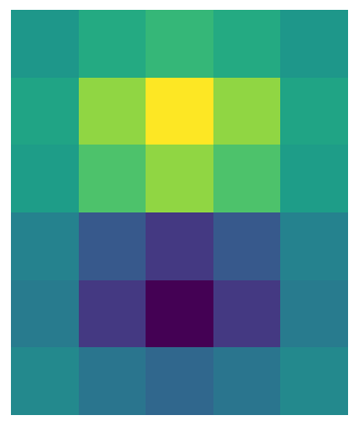
In this part, I additionally smoothed the image using a Gaussian filter, before applying the finite difference operator to the image, applying the same process above to the smoothed image. After this, I convolved the Gaussian operator with the finite difference operator to make a single operator for the smooth + derivative (DoG Filter), and verified that it produced the same results (not shown).


PLACEHOLDER PLACEHOLDER
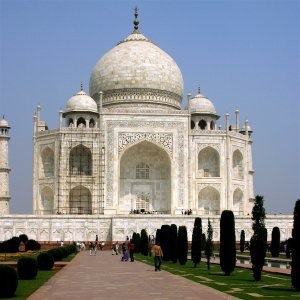
For this part, I sharpened several images by blurring them with a Gaussian filter, and subtracting the blurred image from the original. I applied this to the given Taj Mahal image, as well as a blurry image of Mt. Whitney that I took on a camping trip. Additionally, I blurred the sharpened Taj Mahal image, and applied the sharpening procedure again to the blurred image, with interesting results described below.
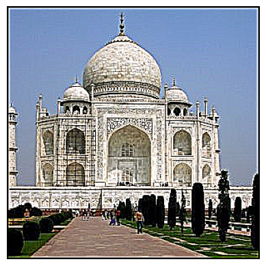
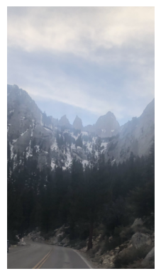
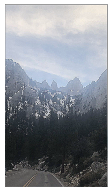
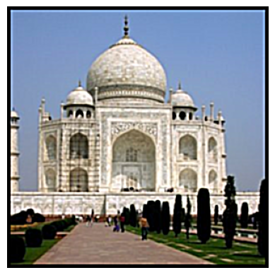
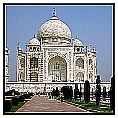
After resharpening the blurred image, it looks sharp in a similar style to the original sharpened image. However, it is missing some image details from the original image, which makes sense, as these details were lost by the blurring of the original image
This part involved taking several pairs of images and producing "hybrid images", or images that look different depending on how close to the screen you view them from. This is done by applying a high-pass filter to one image, applying a low-pass filter to the other image, and averaging the two together.
In the spirit of the example given, I first made a hybrid image of myself and my family's cat, Miso.
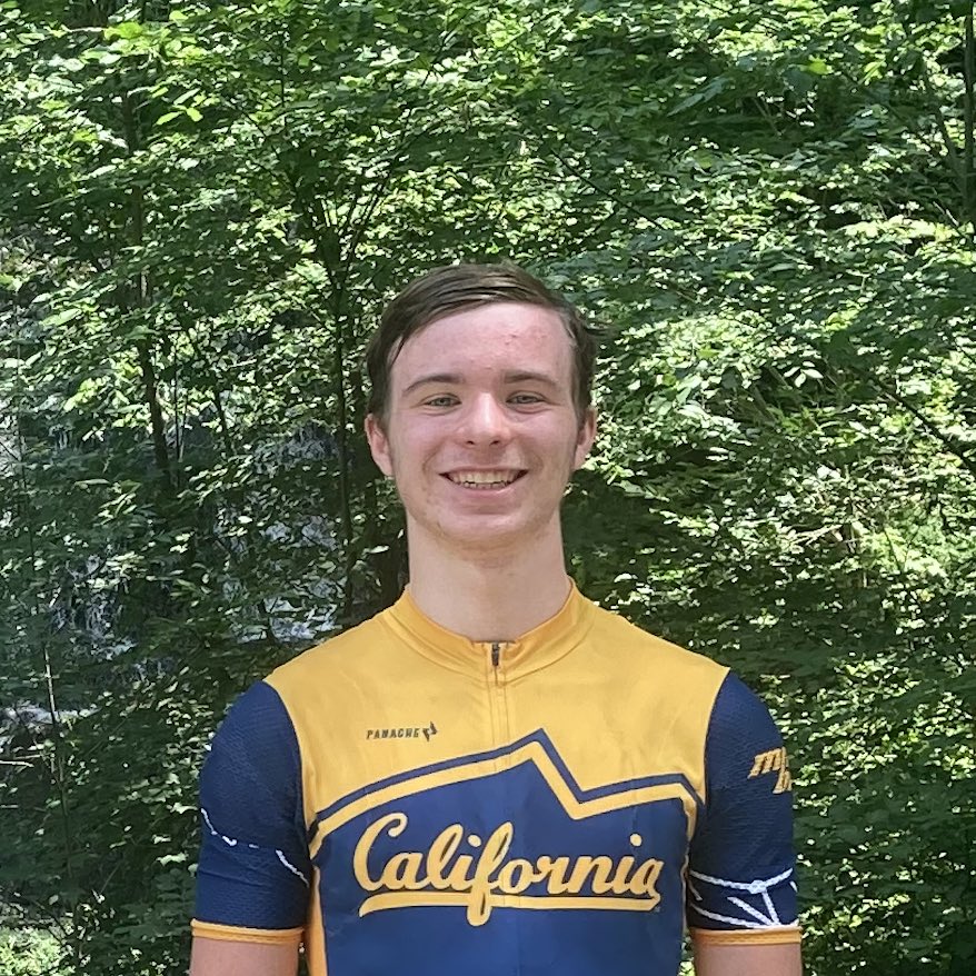
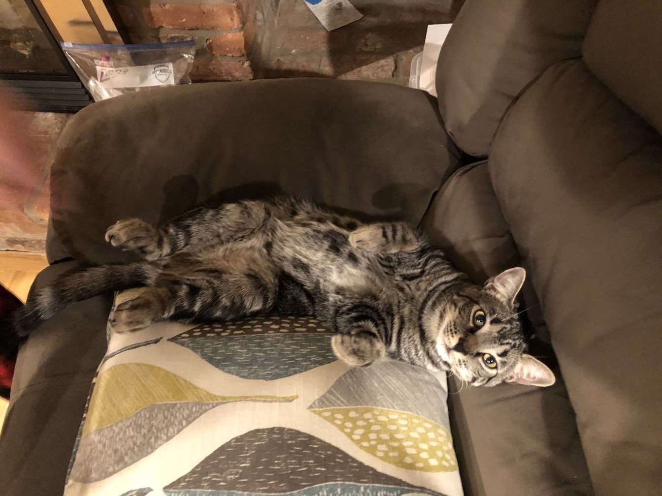
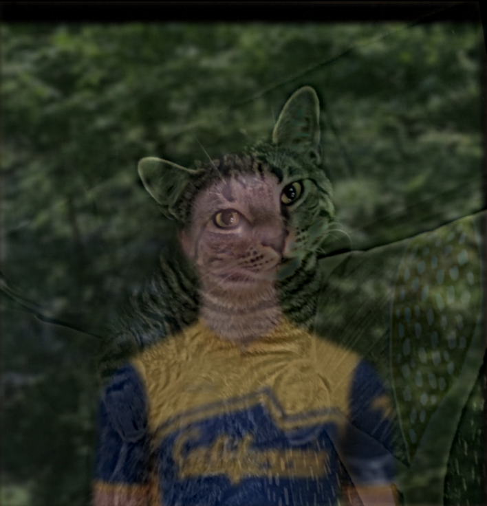
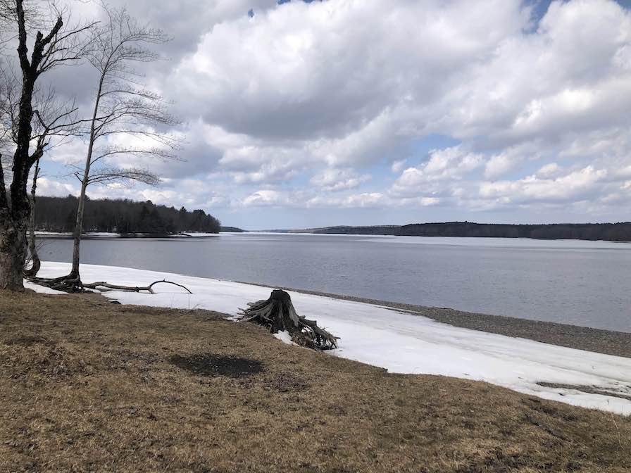
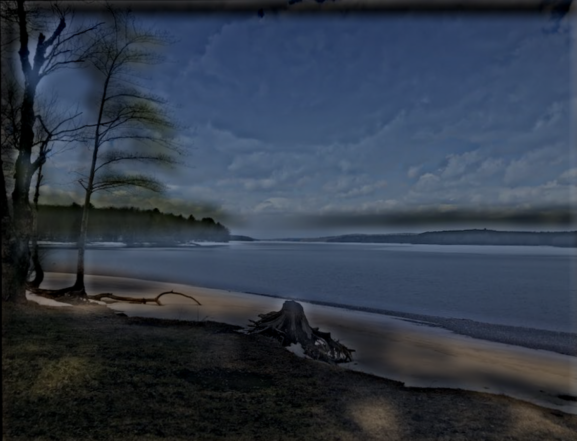
Next, I made a hybrid image of two pictures I took from the same spot at the Salmon River Reservoir in New York, with one of the images being from the summer, and the other from the winter. Notice the snow in the winter image.
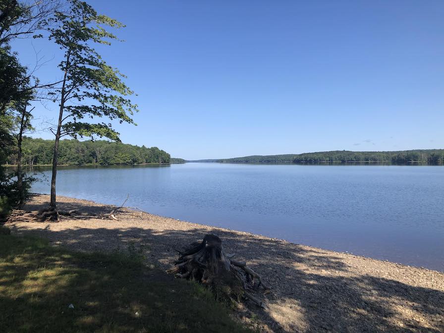
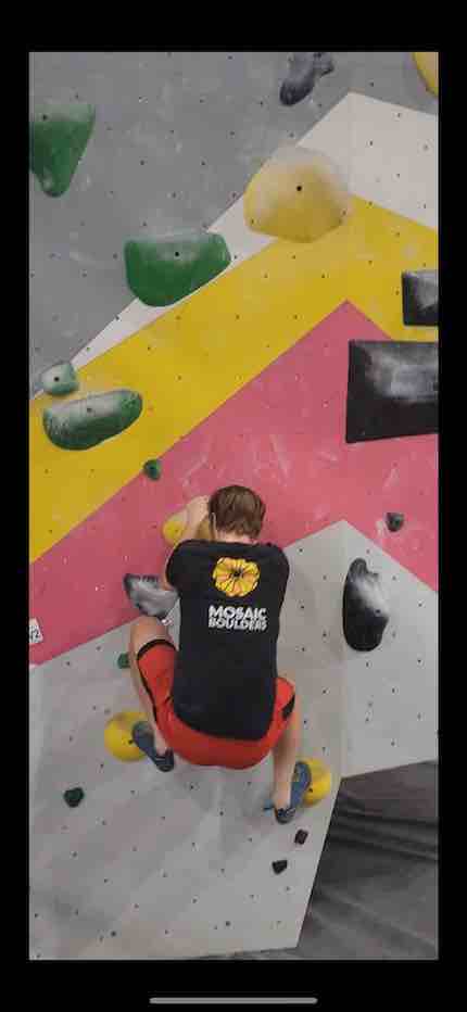
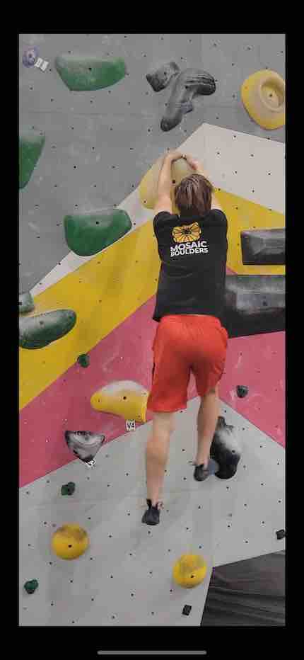
Finally, I tried a hybrid image of two pictures I took of myself doing a jump while rock climbing - with the first picture taken before the jump, and the second picture taken after the jump. This ended up being a failure case - because I am at two different places in each image, you can still see faint signs of both images in the hybrid image no matter where you look at it from.
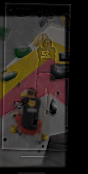
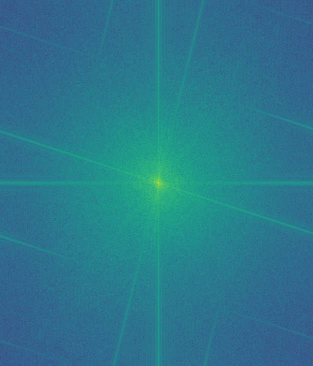
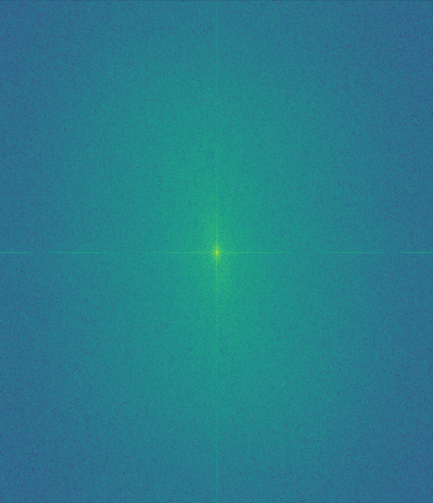
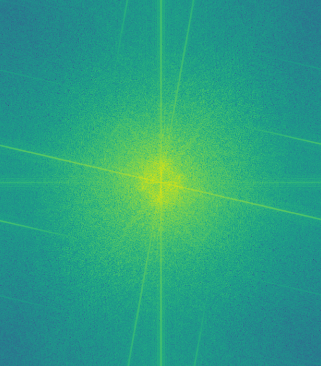
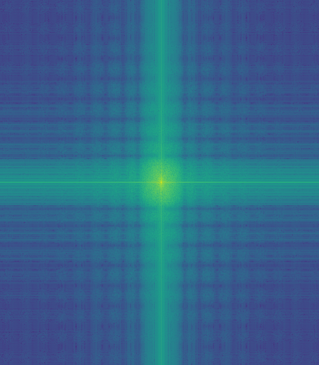
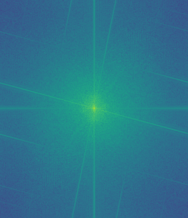
To illustrate the process of a successful hybrid image, I took images of the fourier transform of various parts of the process as applied to the first set of images converted to grayscale.
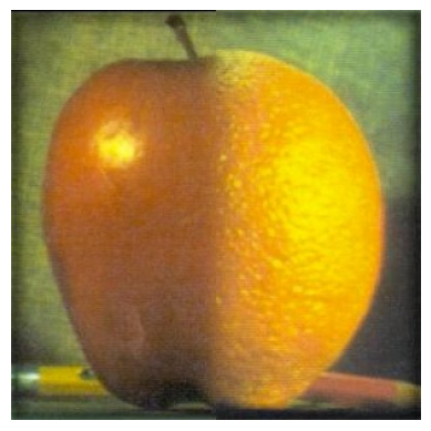
For this section, I implemented the results of a 1983 paper to blend two images together, with the "oraple" (orange + apple) example shown in this part. Specifically, this blending process involved finding Laplacian stacks for each image and taking a mask (for the Oraple example, a simple binary left-right mask) and repeatedly convolving it with a 2D Gaussian. Then, each level of the Laplacian stack is multiplied with the corresponding level of the blurred mask, and all of these multiplied results are added together to get a nicely blended image.
This section illustrates the Laplacian stack of both the apple and orange, and the result of averaging these. The final Oraple image is shown in the next section
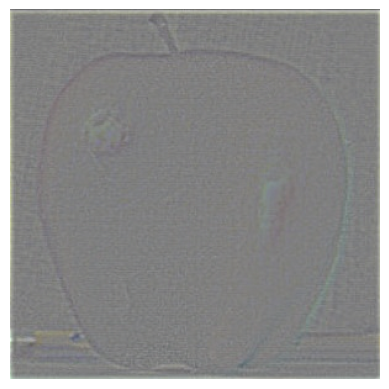
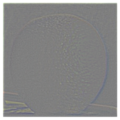
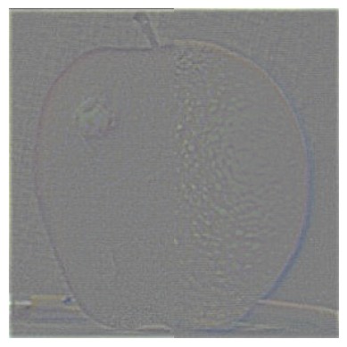
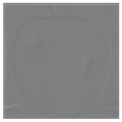
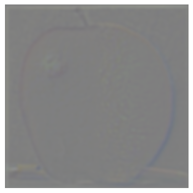
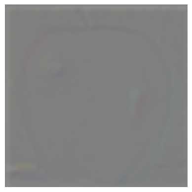
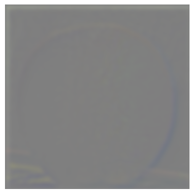
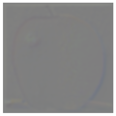
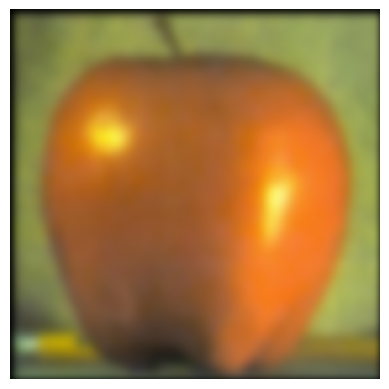
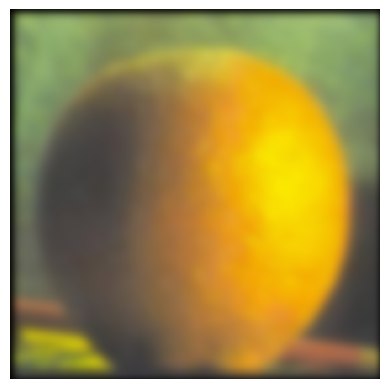
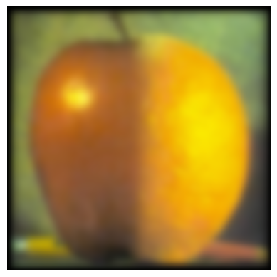
This section illustrates the results of the process described in the previous part, both applied to the Oraple and to several new images, with different masks for the new images.
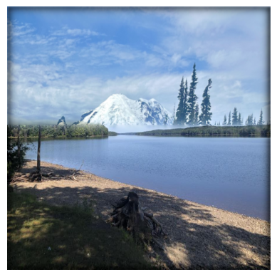
After the Oraple example, I took the same image from the Salmon River Reservoir that I used as part of a hybrid image in 2.2, and blended it with an image of Mt. Rainier, to make it look like Mt. Rainier is behind the reservoir:
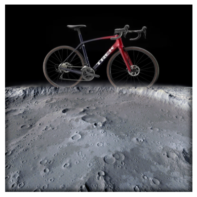
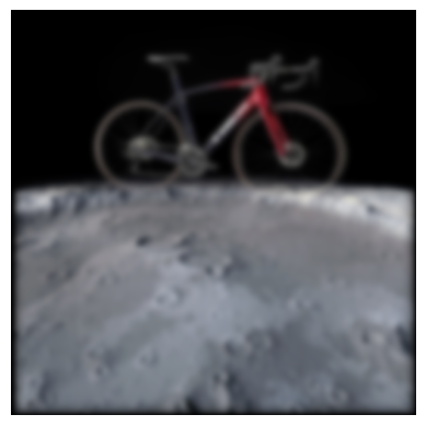
Next, I took an image of a Trek Domane SL5 bike, the same model of road bike that I have, and blended it with an image of the moon:
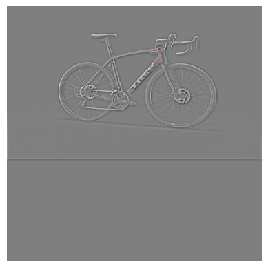
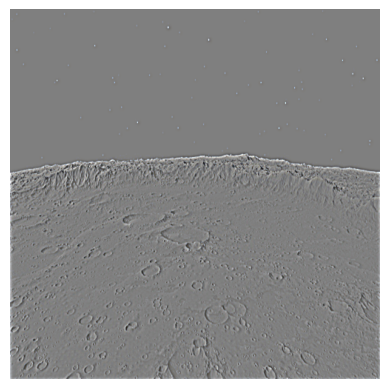
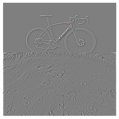
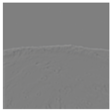
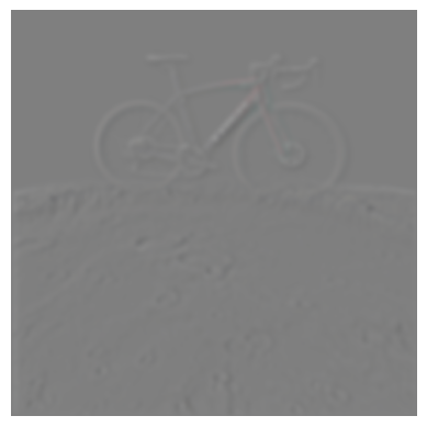
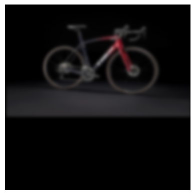
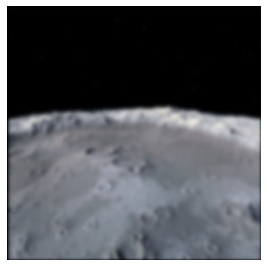
Here are some selected portions of the Laplacian stack for the previous blending:

I had a lot of fun working on this project! The most important thing I learned from this project was that when you apply results from papers like the ones in 2.2 and 2.3-4 and apply them to your own images, it can take a lot of tweaking of parameters to get the results to look good and look similar to the paper results.